February | 2015 | KWANT PRESS

It’s been a while since I looked at variable annuity products so I am writing this post to refresh my own memory as well as provide readers with an overview!

A variable annuity is an insurance product, most often used to provide life insurance. People invest their money and are supposed to receive periodic payments that depend on the performance of the investment portfolio selected. Let’s assume that Mr. A has bought a variable annuity from a life insurance company. The insurance company purchases a basket of equity, bond, and money market instruments on behalf of Mr. A. The basket can be fixed over time or can be rebalanced periodically in order to maintain a target set of weights among the different assets. The insurance company will pay a coupon based on the performance of the basket each year until death. In the event of death the insurance company pays an amount that depends on the value of the basket to the beneficiaries of Mr. A. However the insurance company also guaranties that the coupons will be above some minimum level and also that the death benefit will be at least some specified amount. So the insurance protects Mr. A against the risk of having his income fall below a certain level and provides Mr. A’s beneficiaries with protection in case of his death. With these products, the client also has the right to exit the contract and receive a lump sum based on the value of the basket less a haircut. Depending on the contract, this lump sum can be also floored so that the client will receive at least his initial investment back.

So Mr. A, having invested in a variable annuity, can receive three types of income:

A retirement income equal to the minimum coupon plus a variable amount depending on the performance of the investment portfolio.
At least the guaranteed lump sum in case of death.
A lump sum with a hair cut applied if he exits the contract.

The lump sum is normally calculated based on a maximum drawdown. It is a weighted lookback or a level that depends on the maximum and average value of the variable annuity portfolio since inception.

These life insurance products are generally in demand for many reasons, including providing an extra pension for the purchaser and covering the cost of inheritance tax for the beneficiaries. This overview of variable annuities is a very simplistic one. There are three main risks associated with variable annuities: the client exit risk, the death risk, and the market risk. The first two are actuarial risks. The market risk arising from selling a variable annuity is a complicated structured product.

The insurance company normally uses a bank to cover its market risk, which is the risk that the portfolio income cannot cover the floored level for the lump sum. Both the death and client exit risks can be quantified using deterministic models based on actuarial assumptions or stochastic models.

One of the risks of the variable annuity product is its sensitivity to the correlation between stocks and bonds. When rates go high, they normally have a slightly negative correlation to equities and a strong negative correlation to bond values. So in case of a positive move in rates, both the equity and the bond components of the portfolio will tend to go down in value. This dynamic will magnify the portfolio losses and will need to be taken into account when pricing the put option embedded in the variable annuity.

Mastering risk neutral probabilities took me a while so I thought it worthwhile to share my experience. The risk neutral probability is the probability measure that applies when asset prices are martingales. The expected future value of an asset is equal to its value today. In mathematical terms, assuming that the risk-free rate is zero $( r=0 )$ , we have:

$E[S_t | \Im_0]=S_0$

where $\Im_0$ is the filtration (or the set of scenarios that could happen up to time 0) and $S_t$ is the asset price at time t. In a risk neutral world the expected future value of an asset is its value today. This result is a consequence of the no-arbitrage principle. If the expected future price of the asset is different from its current price, the market would purchase or sell the asset until it reaches the equilibrium level. Hence the risk neutral probability is based on the reachability of an asset.

We know that under the historical probability measure the above equation is untrue. The expected value of the asset can be higher or lower than its current value. Assume that the expected future value of a stock is higher than its value today. In other words, one expects the asset price to increase. Given the risk associated with the asset, however, no one “dares” to purchase it at a higher price.

Hence the historical expectation of an asset is not a sufficient indicator of its price. The risk neutral probability adjusts the expected return of the asset. So the risk neutral probability is nothing more than a linear shift of the historical density; it does not change the variance or correlation, but only shifts the density to a new center.

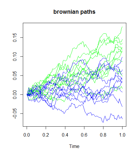
Let’s assume that we have an asset with drift $\mu$ and volatility $\sigma$ . The relationship between a Brownian path in the historical world $( W^{P} )$ and the risk neutral world $( W^{Q} )$ is a shift in the drift:

$W^{P}_T=W^{Q}_T+\frac{\mu-r}{\sigma}T$

Brownian paths in risk neutral and historical world. The green lines are the risk neutral paths , the blue lines are the historical paths. The green process do not seem to be a martingale, but is a martingale in a risk neutral world.