Author Archives: B Moradian

Unknown's avatar

About B Moradian

I am an alumni of Ecole Polytechnique and Sharif University. I am currently working as a quantitative analyst in one Investment Bank in London.

How to build a C++ library package in R

I am building an R package that has Boost and QuantLib dependency. It is a library package, which took me a while to compile in R. I thought it might be interesting to share my experience with others. I came up with the following solution that works for a Windows 64-bit platform. Here are the instructions:

  1. Download and install R from: http://cran.r-project.org/bin/windows/base/
  2. Download and install latest version of Rtools from: http://cran.r-project.org/bin/windows/Rtools/
  3. Download and install MikTex from: http://miktex.org/download
  4. Add to System Environment PATH: to R, example: C:\R-3.1.2\bin; to RTools, example: C:\Rtools\bin;c:\Rtools\gcc-4.6.3\bin;C:\Rtools\gcc-4.6.3\i686-w64-mingw32\bin; to perl, example: to miktex, example: C:\Program Files (x86)\MiKTeX 2.9\miktex\bin; Control Panel -> System -> Advanced System Settings -> Advanced -> Environment Variables Edit path variable by appending paths after ;
  5. Download Boost and build it with Rtools
    1. Unpack loaded code
    2. Open command line Win+R -> cmd.exe
    3. Change current folder to your Boost folder. For example, cd C:\libraries\boost_1_57_0 4. Type command: bootstrap mingw
    4. Type command: b2 toolset=gcc address-model=3. Your compiled libraries are now in stage/lib subfolder
    5. Type command: b2 toolset=gcc address-model=64. Your compiled libraries are now in stage/lib subfolder
    6.  In case you have problems due to missing ml, make sure MASM and MASM64 (ml.exe and ml64.exe) are available in PATH. This should be in the C:\Program Files (x86)\Microsoft Visual Studio path
  6. Download QuantLib and build it with your version of Boost headers. You can download QuantLib from http://quantlib.org/ make sure to download the .tar.gz file. Here we have loaded QuantLib-1.5
    1. open msys and run the following instructions
      1. cd C:/Working/QuantLib
      2. tar xzvf QuantLib-1.4.tar.gz. Also make sure that the path to mingw is set to the one in Rtools
    2. open msys, run the following instructions:
      1. cd C:/Working/QuantLib/QuantLib-1.4
      2. configure CXX=’g++ -m32′ CXXFLAGS=’-g -O2 -std=c++0x’ –with-boost-include=C:/Working/boost/boost_1_57_0 –prefix=C:/Working/QuantLib/QuantLib-1.4
    3. Build the same library for x64 architecture: CXX=’g++ -m64′ CXXFLAGS=’-g -O2 -std=c++0x’ Note that you should have around 5GB of free space for successful compilation
  7. Create a folder for your package
    1. Create three folders: R, man, src
    2. Create or update DESCRIPTION file with information about the package, its author, and link libraries
    3. Copy the code you need to build the function into the src folder
    4. If the original code could be compiled without issues with Rtools compiler (mingw), you should only add dllmain.cpp with defined dllentry
    5. Make a file named NAMESPACE in the root directory. There we define which dlls we need for the package to work (useDynLib) and what we should export from them (export or export pattern). Also we should identify which R packets we should import (import)
  8. R package run:
    1. Write wrapper on R to call function from dll
    2. To make documentation, open R. Type install.packages(‘roxygen2’). Change folder to your package root folder. Type roxygen2::roxygenise().
  9. Create file Makevars.win to build your package library in the windows environment. In this file it is very important to set following the variables: SOURCES, OBJECTS, PKG_CPPFLAGS, PKG_LIBS. These variables will be updated as you continue to develop your code. Of course, you can add additional build targets. SOURCES is an enumeration of all cpp files you need to build your function from the project (including dependencies). You should update this variable whenever you add additional cpp files. OBJECTS is an enumeration of object files compiled from SOURCES. PKG_CPPFLAGS is the set of flags used for code compilation, including paths to include files. Note we also use the -std=c++0x flag for Boost compatibility. Here the $(shell RScript -e Rcpp:::CxxFlags()) command helps access R and Rcpp include files. You should update this variable whenever you add new h or hpp files to build. PKG_LIBS is the set of flags used for code linking, including paths to additional libraries. $(shell RScript -e Rcpp:::LdFlags()) helps to link Rcpp libraries. You should update this variable whenever you require the use of a new library in your code
  10. Prepare environment. For some reason in current version of R, makefile for package uses only gcc for linking. And we need to use g++ to support template functionality of boost %.dll: replace line 216 in \etc\i386\Makeconf and in \etc\x64\Makeconf $(SHLIB_LD) -shared $(DLLFLAGS) -o $@ $*.def $^ $(ALL_LIBS) with $(SHLIB_CXXLD) -shared -o $@ $*.def $^ $(ALL_LIBS) or replace line: CC = $(BINPREF)gcc $(M_ARCH) with CC = $(BINPREF)g++ $(M_ARCH)
  11. If you successfully complete all the previous steps, you can verify your package. Open command line Win+R cmd.exe. Change current folder to your package parent folder. Type: R CMD check

On share repurchase programs

A type of structured product that has become fashionable these days is the structured share repurchase program. When a corporate client wants to buy back its own shares, it normally uses its broker or investment bank to buy shares on the open market. The repurchase program will be announced before the start of the program and the announcement may have an impact on the share price.

In a normal share repurchase program, the broker behaves as an agent and buys a fixed amount per day up to a certain notional amount or number of shares. The amount purchased per day depends on the deadline and the target notional or target number of shares. The deadline for the completion of the repurchase program is often quite important for the corporate client and is normally set before the end of a quarterly accounting period or announcement. Depending on whether the corporate client targets a notional amount or a number of shares, the share repurchase program is called fixed notional or fixed shares.

A new structure proposed by investment banks has recently become popular as it can provide cheaper prices for the corporate client. Under these new structures, the maturity and target number of shares or notional amount are fixed, but the total number of shares that are repurchased can vary. The investment bank has the optionality on how many shares to purchase per day as long as it commits itself to finishing the repurchase program by the deadline and not buying back more than a certain number of shares each day. With such programs the investment bank is able to give a discount to the client. At the same time the investment bank will be paid the volume weighted average price (VWAP) over the period minus the discount. A good trader taking advantage of the daily optionality can beat the VWAP average price. Hence in many circumstances it is desirable for the investment bank to not delta hedge its position and keep the option naked in the book so that it can make money out of daily price movements.

On Dupire local volatility

The Dupire equation for local volatility is surely one of the biggest technological discoveries in the pricing of equity derivatives. It has significantly changed how the market analyses and manages the risk of structured products. Despite having many deficiencies, the model is being used in an industrial way. By industrial, I really mean like a factory. Although it doesn’t account for many of the associated risks, the local volatility model is the benchmark for pricing any structured product. The local volatility model is also the most widely used approach for risk management. But why is the local volatility model so widely used? The main reasons are that the model is very easy to implement and the simulations using the model are so precise. Nevertheless the local volatility model has many deficiencies and does not accurately price products with non-European options. Furthermore the standard Dupire formula is not the best choice for actually implementing the model. Instead Jim Gatheral’s implementation of local volatility is surely more practical for the simple reason that we tend to see prices as a function of implied volatilities rather than of actual vanilla option prices. Gatheral suggests the following formulation:

\sigma ^2 ( K,T) = \frac{\frac{\partial \omega}{\partial T}}{1-\frac{k}{\omega}\frac{\partial \omega}{\partial k} +\frac{1}{4}\left ( -\frac{1}{4} -\frac{1}{\omega} +\frac{k^2}{\omega^2}\right ) \left ( \frac{\partial \omega}{\partial k} \right )^2 +\frac{1}{2}\frac{\partial^2 \omega}{\partial k^2} }

where \sigma ^2 ( K,T) is the local variance, K is the strike, and T is the maturity. k= ln \left ( \frac {K}{F_T} \right ) is the log moneyness strike where F_T is the forward and \omega= \sigma_{BS}^2 ( K,T)T is the implied total variance. As seen in the above equation, the local volatility is a function of the implied volatility rather than call/put prices. This approach is much more useful in practice.

On variable annuities

It’s been a while since I looked at variable annuity products so I am writing this post to refresh my own memory as well as provide readers with an overview!

A variable annuity is an insurance product, most often used to provide life insurance. People invest their money and are supposed to receive periodic payments that depend on the performance of the investment portfolio selected. Let’s assume that Mr. A has bought a variable annuity from a life insurance company. The insurance company purchases a basket of equity, bond, and money market instruments on behalf of Mr. A. The basket can be fixed over time or can be rebalanced periodically in order to maintain a target set of weights among the different assets. The insurance company will pay a coupon based on the performance of the basket each year until death. In the event of death the insurance company pays an amount that depends on the value of the basket to the beneficiaries of Mr. A. However the insurance company also guaranties that the coupons will be above some minimum level and also that the death benefit will be at least some specified amount. So the insurance protects Mr. A against the risk of having his income fall below a certain level and provides Mr. A’s beneficiaries with protection in case of his death. With these products, the client also has the right to exit the contract and receive a lump sum based on the value of the basket less a haircut. Depending on the contract, this lump sum can be also floored so that the client will receive at least his initial investment back.

So Mr. A, having invested in a variable annuity, can receive three types of income:

  1. A retirement income equal to the minimum coupon plus a variable amount depending on the performance of the investment portfolio.
  2. At least the guaranteed lump sum in case of death.
  3. A lump sum with a hair cut applied if he exits the contract.

The lump sum is normally calculated based on a maximum drawdown. It is a weighted lookback or a level that depends on the maximum and average value of the variable annuity portfolio since inception.

These life insurance products are generally in demand for many reasons, including providing an extra pension for the purchaser and covering the cost of inheritance tax for the beneficiaries. This overview of variable annuities is a very simplistic one. There are three main risks associated with variable annuities: the client exit risk, the death risk, and the market risk. The first two are actuarial risks. The market risk arising from selling a variable annuity is a complicated structured product.

The insurance company normally uses a bank to cover its market risk, which is the risk that the portfolio income cannot cover the floored level for the lump sum. Both the death and client exit risks can be quantified using deterministic models based on actuarial assumptions or stochastic models.

One of the risks of the variable annuity product is its sensitivity to the correlation between stocks and bonds. When rates go high, they normally have a slightly negative correlation to equities and a strong negative correlation to bond values. So in case of a positive move in rates, both the equity and the bond components of the portfolio will tend to go down in value. This dynamic will magnify the portfolio losses and will need to be taken into account when pricing the put option embedded in the variable annuity.

What is the risk neutral measure?

Mastering risk neutral probabilities took me a while so I thought it worthwhile to share my experience. The risk neutral probability is the probability measure that applies when asset prices are martingales. The expected future value of an asset is equal to its value today. In mathematical terms, assuming that the risk-free rate is zero ( r=0 ) , we have:

E[S_t | \Im_0]=S_0

where \Im_0 is the filtration (or the set of scenarios that could happen up to time 0) and S_t 
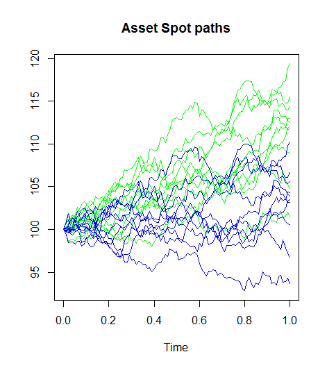
is the asset price at time t. In a risk neutral world the expected future value of an asset is its value today. This result is a consequence of the no-arbitrage principle. If the expected future price of the asset is different from its current price, the market would purchase or sell the asset until it reaches the equilibrium level. Hence the risk neutral probability is based on the reachability of an asset.

We know that under the historical probability measure the above equation is untrue. The expected value of the asset can be higher or lower than its current value. Assume that the expected future value of a stock is higher than its value today. In other words, one expects the asset price to increase. Given the risk associated with the asset, however, no one “dares” to purchase it at a higher price.

Hence the historical expectation of an asset is not a sufficient indicator of its price. The risk neutral probability adjusts the expected return of the asset. So the risk neutral probability is nothing more than a linear shift of the historical density; it does not change the variance or correlation, but only shifts the density to a new center.

Let’s assume that we have an asset with drift \mu and volatility \sigma
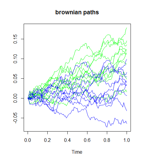
. The relationship between a Brownian path in the historical world ( W^{P} ) and the risk neutral world ( W^{Q} ) is a shift in the drift:

W^{P}_T=W^{Q}_T+\frac{\mu-r}{\sigma}T

Brownian paths in risk neutral and historical world

Brownian paths in risk neutral and historical world. The green lines are the risk neutral paths , the blue lines are the historical paths. The green process do not seem to be a martingale, but is a martingale in a risk neutral world.

Asset paths in a risk neutral and historical world

Asset paths in a risk neutral and historical world

This blog post will be continued….